40 show data labels excel

Where is labels in excel? - ler.jodymaroni.com How do I show percentage data labels in Excel? Right click the pie chart again and select Format Data Labels from the right-clicking menu. 4. In the opening Format Data Labels pane, check the Percentage box and uncheck the Value box in the Label Options section. Then the percentages are shown in the pie chart as below screenshot shown. How Do I Create Avery Labels From Excel? - Ink Saver 07.03.2022 · When you have to create numerous labels with different data sets, you must first capture all the details in a spreadsheet. You could import the data to a tool such as Microsoft Word for labeling or mail merging from the spreadsheet. However, Word and other Microsoft products don't offer much when it comes to labeling. These […]

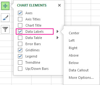
Change the format of data labels in a chart To get there, after adding your data labels, select the data label to format, and then click Chart Elements > Data Labels > More Options. To go to the appropriate area, click one of the four icons ( Fill & Line, Effects, Size & Properties ( Layout & Properties in Outlook or Word), or Label Options) shown here.

Show data labels excel

How to Rename a Data Series in Microsoft Excel - How-To Geek Jul 27, 2020 · A data series in Microsoft Excel is a set of data, shown in a row or a column, which is presented using a graph or chart. To help analyze your data, you might prefer to rename your data series. Rather than renaming the individual column or row labels, you can rename a data series in Excel by editing the graph or chart. 5 New Charts to Visually Display Data in Excel 2019 - dummies 26.08.2021 · Select the data and labels and then click Insert → Maps → Filled Map. Wait a few seconds for the map to load. Resize and format as desired. For example, you could apply one of the chart styles from the Chart Tools Design tab. To add data labels to the chart, choose Chart Tools Design → Add Chart Element → Data Labels → Show. Pouring ... Add a DATA LABEL to ONE POINT on a chart in Excel Steps shown in the video above: Click on the chart line to add the data point to. All the data points will be highlighted. Click again on the single point that you want to add a data label to. Right-click and select ' Add data label ' This is the key step! Right-click again on the data point itself (not the label) and select ' Format data label '.

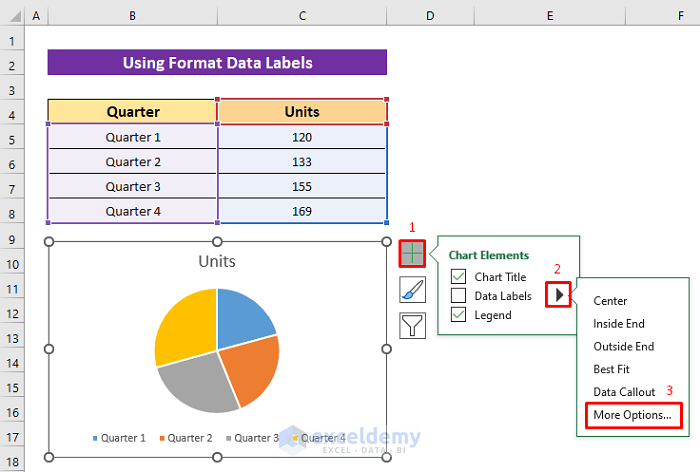
Show data labels excel. how to add data labels into Excel graphs - storytelling with data You can download the corresponding Excel file to follow along with these steps: Right-click on a point and choose Add Data Label. You can choose any point to add a label—I'm strategically choosing the endpoint because that's where a label would best align with my design. Excel defaults to labeling the numeric value, as shown below. How to Make a Pie Chart in Excel & Add Rich Data Labels to 08.09.2022 · A pie chart is used to showcase parts of a whole or the proportions of a whole. There should be about five pieces in a pie chart if there are too many slices, then it’s best to use another type of chart or a pie of pie chart in order to showcase the data better. In this article, we are going to see a detailed description of how to make a pie chart in excel. How to hide zero data labels in chart in Excel? - ExtendOffice If you want to hide zero data labels in chart, please do as follow: 1. Right click at one of the data labels, and select Format Data Labels from the context menu. See screenshot: 2. In the Format Data Labels dialog, Click Number in left pane, then select Custom from the Category list box, and type #"" into the Format Code text box, and click Add button to add it to Type list box. How to show data label in "percentage" instead of - Microsoft Community Select Format Data Labels Select Number in the left column Select Percentage in the popup options In the Format code field set the number of decimal places required and click Add. (Or if the table data in in percentage format then you can select Link to source.) Click OK Regards, OssieMac Report abuse 8 people found this reply helpful ·

Displaying Large Numbers in K (thousands) or M (millions) in Excel Right Click, and choose Custom Formatting. You can also choose Number Formatting from the Home Ribbon, or simply press the shortcut [Ctrl] + 1. Go to Custom, and key in 0, "K" in the place where it says General. Now close the Format Cells popup window. Custom Number Format Popup in Microsoft Excel. How to use data labels in a chart - YouTube Excel charts have a flexible system to display values called "data labels". Data labels are a classic example a "simple" Excel feature with a huge range of o... Fix Excel Pivot Table Missing Data Field Settings - Contextures Excel … Aug 31, 2022 · Show Missing Data. To show missing data, such as new products, you can add one or more dummy records to the pivot table, to force the items to appear. For example, to include a new product -- Paper -- in the pivot table, even if it has not yet been sold: In the source data, add a record with Paper as the product, and 0 as the quantity; Refresh ... Edit titles or data labels in a chart - support.microsoft.com The first click selects the data labels for the whole data series, and the second click selects the individual data label. Right-click the data label, and then click Format Data Label or Format Data Labels. Click Label Options if it's not selected, and then select the Reset Label Text check box. Top of Page

How to Use Cell Values for Excel Chart Labels - How-To Geek Mar 12, 2020 · Make your chart labels in Microsoft Excel dynamic by linking them to cell values. When the data changes, the chart labels automatically update. In this article, we explore how to make both your chart title and the chart data labels dynamic. We have the sample data below with product sales and the difference in last month’s sales. How to format axis labels as thousands/millions in Excel? - ExtendOffice 3. Close dialog, now you can see the axis labels are formatted as thousands or millions. Tip: If you just want to format the axis labels as thousands or only millions, you can type #,"K" or #,"M" into Format Code textbox and add it. Add or remove data labels in a chart - support.microsoft.com Data labels make a chart easier to understand because they show details about a data series or its individual data points. For example, in the pie chart below, without the data labels it would be difficult to tell that coffee was 38% of total sales. Depending on what you want to highlight on a chart, you can add labels to one series, all the ... Find, label and highlight a certain data point in Excel scatter graph Select the Data Labels box and choose where to position the label. By default, Excel shows one numeric value for the label, y value in our case. To display both x and y values, right-click the label, click Format Data Labels…, select the X Value and Y value boxes, and set the Separator of your choosing: Label the data point by name

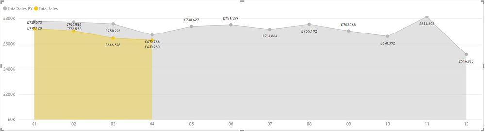
Excel Charts: Dynamic Label positioning of line series

Custom Chart Data Labels In Excel With Formulas - How To Excel At Excel Follow the steps below to create the custom data labels. Select the chart label you want to change. In the formula-bar hit = (equals), select the cell reference containing your chart label's data. In this case, the first label is in cell E2. Finally, repeat for all your chart laebls.

How to hide zero data labels in chart in Excel?

How to add or move data labels in Excel chart? - ExtendOffice In Excel 2013 or 2016. 1. Click the chart to show the Chart Elements button . 2. Then click the Chart Elements, and check Data Labels, then you can click the arrow to choose an option about the data labels in the sub menu. See screenshot: In Excel 2010 or 2007. 1. click on the chart to show the Layout tab in the Chart Tools group. See ...

How to Make Pie Chart with Labels both Inside and Outside ...

Format Data Labels in Excel- Instructions - TeachUcomp, Inc. To format data labels in Excel, choose the set of data labels to format. To do this, click the "Format" tab within the "Chart Tools" contextual tab in the Ribbon. Then select the data labels to format from the "Chart Elements" drop-down in the "Current Selection" button group. Then click the "Format Selection" button that ...

How can I format the data labels so that they will show as ...

How to Show Percentage Change in Excel Graph (2 Ways) 31.05.2022 · This article will illustrate how to show the percentage change in an Excel graph. Using an Excel graph can present you the relation between the data in an eye-catching way. Showing partial numbers as percentages is easy to understand while analyzing data. In the following dataset, we have a company’s Profit during the period March to September.

excel - How to show series-Legend label name in data labels ...

Excel, giving data labels to only the top/bottom X% values 1) Create a data set next to your original series column with only the values you want labels for (again, this can be formula driven to only select the top / bottom n values). See column D below. 2) Add this data series to the chart and show the data labels. 3) Set the line color to No Line, so that it does not appear! 4) Volia! See Below! Share

Change the format of data labels in a chart

How to add data labels from different column in an Excel chart? Right click the data series, and select Format Data Labels from the context menu. 3. In the Format Data Labels pane, under Label Options tab, check the Value From Cells option, select the specified column in the popping out dialog, and click the OK button. Now the cell values are added before original data labels in bulk. 4.

How to show data labels in PowerPoint and place them ...

How to create a chart with both percentage and value in Excel? After installing Kutools for Excel, please do as this:. 1.Click Kutools > Charts > Category Comparison > Stacked Chart with Percentage, see screenshot:. 2.In the Stacked column chart with percentage dialog box, specify the data range, axis labels and legend series from the original data range separately, see screenshot:. 3.Then click OK button, and a prompt message is popped out to remind you ...

Is there a way to add data labels as percentages on the ...

How to Create Mailing Labels in Word from an Excel List 09.05.2019 · Before you can transfer the data from Excel to your labels in Word, you must connect the two. Back in the “Mailings” tab in the Word document, select the “Select Recipients” option. A drop-down menu will appear. Select “Use an Existing List.” Windows File Explorer will appear. Use it to locate and select your mailing list file. With the file selected, click “Open.” The ...

Apply Custom Data Labels to Charted Points - Peltier Tech

Excel tutorial: How to use data labels Generally, the easiest way to show data labels to use the chart elements menu. When you check the box, you'll see data labels appear in the chart. If you have more than one data series, you can select a series first, then turn on data labels for that series only. You can even select a single bar, and show just one data label.

data visualization - How do you put values over a simple bar ...

How to Show Percentage in Pie Chart in Excel? - GeeksforGeeks Jun 29, 2021 · It can be observed that the pie chart contains the value in the labels but our aim is to show the data labels in terms of percentage. Show percentage in a pie chart: The steps are as follows : Select the pie chart. Right-click on it. A pop-down menu will appear. Click on the Format Data Labels option. The Format Data Labels dialog box will appear.

How To Show Or Hide Data Labels On MS Excel? | My Windows Hub

Use Excel Data Validation for Entering Dates - Contextures Excel … 13.05.2022 · How to use Excel data validation rules to prevent invalid dates from being entered ... Show a drop down list of valid dates (List option) Create a rule in a custom formula (Custom option) Written instructions, and the sample file, are below the video. Limit Entries to Specific Date Range. In this example, employees will fill in a Vacation Request Form for the year 2017. In cell …

This is how you can add data labels in Power BI [EASY STEPS]

How to Add Data Labels in Excel - Excelchat | Excelchat In Excel 2013 and the later versions we need to do the followings; Click anywhere in the chart area to display the Chart Elements button Figure 5. Chart Elements Button Click the Chart Elements button > Select the Data Labels, then click the Arrow to choose the data labels position. Figure 6. How to Add Data Labels in Excel 2013 Figure 7.

Add or remove data labels in a chart

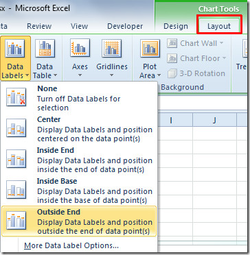
Adding Data Labels to Your Chart (Microsoft Excel) - ExcelTips (ribbon) Select the position that best fits where you want your labels to appear. To add data labels in Excel 2013 or later versions, follow these steps: Activate the chart by clicking on it, if necessary. Make sure the Design tab of the ribbon is displayed. (This will appear when the chart is selected.) Click the Add Chart Element drop-down list.

Total of chart series – Excel kitchenette

How to Add Data Labels to an Excel 2010 Chart - dummies On the Chart Tools Layout tab, click Data Labels→More Data Label Options. The Format Data Labels dialog box appears. You can use the options on the Label Options, Number, Fill, Border Color, Border Styles, Shadow, Glow and Soft Edges, 3-D Format, and Alignment tabs to customize the appearance and position of the data labels.

How to Use Cell Values for Excel Chart Labels

Excel charts: how to move data labels to legend @Matt_Fischer-Daly . You can't do that, but you can show a data table below the chart instead of data labels: Click anywhere on the chart. On the Design tab of the ribbon (under Chart Tools), in the Chart Layouts group, click Add Chart Element > Data Table > With Legend Keys (or No Legend Keys if you prefer)

How to Add Data Labels to an Excel 2010 Chart - dummies

How to Change Excel Chart Data Labels to Custom Values? - Chandoo.org First add data labels to the chart (Layout Ribbon > Data Labels) Define the new data label values in a bunch of cells, like this: Now, click on any data label. This will select "all" data labels. Now click once again. At this point excel will select only one data label. Go to Formula bar, press = and point to the cell where the data label ...

How To Show Or Hide Data Labels On MS Excel? | My Windows Hub

to display top 5 data labels on graph [SOLVED] Re: to display top 5 data labels on graph. Also, I noticed your sum column ("total") is returning errors. I don't see why you would want to do this, and in fact I'm not even sure why excel wanted to do this to begin with. if you run C3+D3 when those cells are empty, excel should return 0. So I got rid of the error, and that way, you can use the ...

How to Add Axis Labels to a Chart in Excel | CustomGuide

Move data labels - support.microsoft.com Right-click the selection > Chart Elements > Data Labels arrow, and select the placement option you want. Different options are available for different chart types. For example, you can place data labels outside of the data points in a pie chart but not in a column chart.

How to Add and Remove Chart Elements in Excel

How to add data labels in excel to graph or chart (Step-by-Step) Add data labels to a chart. 1. Select a data series or a graph. After picking the series, click the data point you want to label. 2. Click Add Chart Element Chart Elements button > Data Labels in the upper right corner, close to the chart. 3. Click the arrow and select an option to modify the location. 4.

how to add data labels into Excel graphs — storytelling with data

How to add a line in Excel graph: average line, benchmark, etc. Select the last data point on the line and add a data label to it as discussed in the previous tip. Click on the label to select it, then click inside the label box, delete the existing value and type your text: Hover over the label box until your mouse pointer changes to a four-sided arrow, and then drag the label slightly above the line:

Adapting charts – empower® Support

How to Add Total Data Labels to the Excel Stacked Bar Chart 03.04.2013 · For stacked bar charts, Excel 2010 allows you to add data labels only to the individual components of the stacked bar chart. The basic chart function does not allow you to add a total data label that accounts for the sum of the individual components. Fortunately, creating these labels manually is a fairly simply process.

How can I hide 0% value in data labels in an Excel Bar Chart ...

Add a DATA LABEL to ONE POINT on a chart in Excel Steps shown in the video above: Click on the chart line to add the data point to. All the data points will be highlighted. Click again on the single point that you want to add a data label to. Right-click and select ' Add data label ' This is the key step! Right-click again on the data point itself (not the label) and select ' Format data label '.

Move data labels

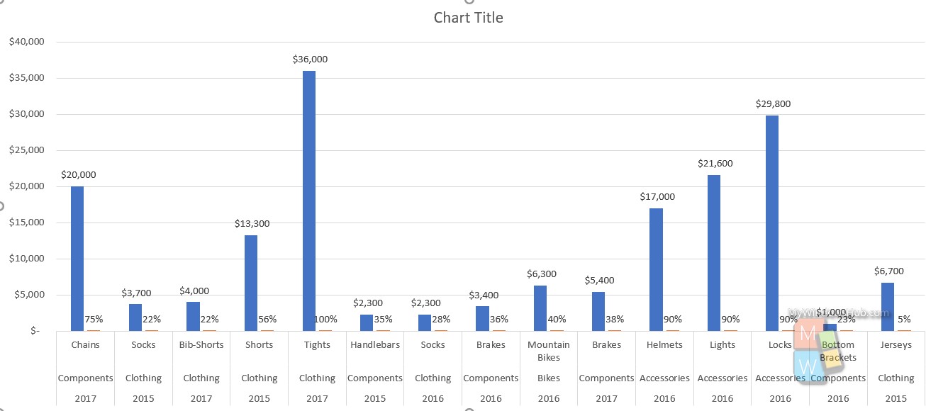
5 New Charts to Visually Display Data in Excel 2019 - dummies 26.08.2021 · Select the data and labels and then click Insert → Maps → Filled Map. Wait a few seconds for the map to load. Resize and format as desired. For example, you could apply one of the chart styles from the Chart Tools Design tab. To add data labels to the chart, choose Chart Tools Design → Add Chart Element → Data Labels → Show. Pouring ...